TL;DR
- Start with readable Python and optimize only when the program is actually too slow.
- Let a coding agent profile the program and move the measured hot path through one implementation stage at a time.
- Keep a known-good implementation and a benchmark harness, then validate every new stage against them.
- My example reaches a 5,290x faster search kernel, but the fastest kernel is not the fastest complete program.
- The implementations, reproduction prompts, harness and raw measurements are in
agentic_speed.
This has become one of my favorite agentic coding design patterns. I have been using it successfully for the past couple of months in reverse engineering, cryptographic tooling, financial backtesting and other compute-heavy local work. I write the straightforward implementation first, keep it while it is fast enough, and involve a coding agent only when a real workload makes the cost visible.
The agent then helps me climb gradually. It can profile the program, optimize the Python hot loop, partition independent work, extract a stable native kernel, remove the Python control plane or move a massively parallel loop to the GPU. I do not need to decide at the beginning that a project is now a C++ project, nor do I have to jump from a Python prototype directly into Metal.
clear, known-good Python
           |
           v
   too slow in practice? ---- no ----> stop
           |
          yes
           v
 profile -> change one hot path -> validate -> measure
                 ^                         |
                 +------ still slow ------+
This is much easier with a coding agent than it used to be. Codex is the concrete agent I used for the example in this post, but the pattern is not product-specific. The useful capability is the loop: inspect the real code, make a bounded change, run the compiler and harness, study the result, and repeat. OpenAI describes a similar use case as using Codex in a scored improvement loop. Here the score is not an abstract eval. It is correctness first, then measured search and wall time.
A benchmark made for the ladder
I built agentic_speed to make the pattern concrete. It solves one deliberately synthetic reverse-engineering problem five ways: recover a low-entropy XTEA key from a recognizable firmware header.
The fictional firmware format begins with the eight ASCII bytes FWPKG01!. An observer knows this plaintext header and has captured its encrypted form. The device nominally uses a 128-bit XTEA key, but provisions it terribly: only the low 20 bits of the first 32-bit word vary, while the other 108 bits are fixed to zero.
known firmware package

  plaintext header     46 57 50 4b 47 30 31 21
                       "F  W  P  K  G  0  1  !"
                              |
                              | XTEA
                              v
  captured ciphertext  e3 ad 41 70 e9 4a 82 88
                              |
                              v
  try K = [candidate, 0, 0, 0], candidate in [0, 2^20)
                              |
                              v
  recovered key        0x0001a2b3
This does not break XTEA. It demonstrates what happens when a system places only 20 bits of entropy into a 128-bit key type and supplies a cheap known-plaintext oracle. The repository’s challenge documentation specifies the byte order, key layout, round convention and expected result. It also links the original Needham-Wheeler XTEA report.
The workload is useful because it is small enough to understand and large enough to expose the execution model. Each candidate performs 32 XTEA cycles of shifts, XORs, additions and subtractions. Candidates are independent. The program always scans the complete requested keyspace, even after finding the key, and accepts only one match. That prevents a lucky key position or an agent-added early exit from masquerading as an optimization.
The same input format, answer, full-scan rule, command-line options and versioned JSON fields survive every implementation. That continuity is the important part of the design pattern. An optimization is not accepted merely because it is fast; it must still perform the same work and produce the same result.
What the agent changes
Before coding agents, I could already have written all five implementations. The friction was in the transitions. Moving a Python loop into a dynamic library means writing a C ABI, defining fixed-width types on both sides, configuring the compiler, checking ownership and deciding which work crosses the boundary. Metal adds an Objective-C++ host, shader compilation, pipeline setup, buffers, dispatch geometry and GPU error handling. Each unfamiliar boundary makes a promising experiment easier to postpone.
An agent reduces that transition cost. It can read the baseline and tests, identify the loop that dominates the profile, preserve the surrounding interface, implement the next stage, run the harness and respond to compiler or test failures. I still choose the constraints and review the result, but I no longer have to reload every toolchain detail into my head before learning whether the idea is worthwhile.
The prompt matters. “Make this faster” leaves too many ways to cheat, including doing less work. I prefer a bounded contract like this:
Profile the current implementation and identify the measured hot path.

Preserve:
- the input and output interfaces
- the complete workload and range boundaries
- the known-good result and error behavior
- the benchmark's setup and search timing definitions

Change only the named performance boundary for this iteration.
Validate the new implementation against the reference harness.
Report search time, end-to-end wall time, and any new maintenance cost.
Stop if the current stage is fast enough for the stated workload.
That contract turns the agent into an iterative performance engineer instead of a code translator. The exact prompts used to reproduce each step live beside the implementations in the repository’s stage descriptions.
The five stages
The ladder is a menu, not a maturity model. A program that stays at the first stage because it finishes in 200 milliseconds is not less engineered than a GPU program. It has simply already met its requirement.
00  readable Python
          |
01  specialized + parallel Python
          |
02  Python control plane + native kernel
          |
03  standalone native program
          |
04  GPU compute kernel

At every arrow: same work -> same answer -> new measurement
Stage 00: readable Python
The baseline solver is ordinary scalar Python. For every candidate it creates a four-word key tuple, calls a reusable decryption function, converts the result back to bytes and compares it with the known header. It is deliberately readable, not deliberately bad.
This distinction matters. A baseline should be code I trust and can explain. It becomes the oracle for later implementations, so sabotaging it with artificial sleeps or absurd data structures would make every speedup meaningless. On the M1 Pro publication run, this version scans 1,048,576 candidates in a median 16.62 seconds.
When a larger application is slow, I first ask the agent to measure it with an appropriate profiler. Python’s cProfile is a convenient deterministic starting point, although sampling profilers are often less intrusive for long-running systems. The goal is not to collect an impressive flame graph. It is to identify whether the suspected loop actually deserves attention.
Stage 01: better and parallel Python
The first optimization stays in the standard library. The agent keeps ciphertext and plaintext as integers, removes tuple construction and byte conversion from the candidate loop, and specializes key lookup for the known sparse layout. It then partitions the range across a reusable multiprocessing pool.
candidate range [0, 2^20)

  worker 0  [        0,   131072) --+
  worker 1  [   131072,   262144)   |
  worker 2  [   262144,   393216)   |
  worker 3  [   393216,   524288)   +--> reduce matches
  worker 4  [   524288,   655360)   |    and examined count
  worker 5  [   655360,   786432)   |
  worker 6  [   786432,   917504)   |
  worker 7  [   917504,  1048576) --+
The pool uses macOS’s explicit spawn context. The Python documentation notes that spawn starts a fresh interpreter, so process creation and import work are real costs. The solver warms the pool before its internal search timer, while the outer wall timer still sees the complete subprocess.
This stage is already useful: median M1 search time falls from 16.62 seconds to 2.81 seconds, a 5.91x improvement, without introducing a native language or third-party dependency. Sometimes this is where I stop.
Stage 02: Python with one coarse native kernel
If interpreter overhead remains inside every round of the hot loop, adding more Python workers does not remove it. The next stage keeps Python for argument parsing, fixture loading, validation and JSON output, but moves the exhaustive search into C++20.
Python: parse -> validate -> prepare result objects
                         |
                         | one typed C ABI call
                         v
C++: partition -> thread -> search -> join -> reduce
                         |
                         v
Python: verify examined count -> emit JSON
The word “one” is important. Crossing an FFI boundary for every candidate would replace Python loop overhead with call overhead. Instead, ctypes makes one call into an extern "C" function. The native side creates threads, processes the complete range and returns the smallest match, match count and examined count through fixed-width outputs.
This is an attractive architecture when most of an application benefits from Python’s ergonomics and only a stable kernel needs native speed. Rust could serve at the same stage behind a C-compatible ABI; I used C++ here, and all measurements in this post are for that implementation. On the M1 Pro, the search itself falls to 19.32 milliseconds. The complete subprocess takes 64.41 milliseconds because Python startup, parsing, library loading and process overhead have not disappeared.
Stage 03: a native program
The standalone C++ stage removes Python and ctypes while preserving the same command-line and JSON contract. It parses the challenge, starts the same style of worker threads, reduces the same complete results and emits the same fields.
Its M1 search median is 18.36 milliseconds, close to the hybrid kernel’s 19.32 milliseconds. That near-plateau is useful evidence: Python was no longer in the timed hot path at stage two. Removing it mainly changes the complete process, which drops from 64.41 to 22.81 milliseconds.
A full native program is therefore not automatically the next correct step. If the Python application is a long-lived process that calls the kernel many times, interpreter startup may be irrelevant and the hybrid design may be easier to maintain. If it is a short-lived command-line tool invoked thousands of times, 40 milliseconds of orchestration may matter. The workload chooses.
Rust is also a reasonable option at this stage. Its official FFI guidance describes the same kind of C boundary needed for a hybrid, while a standalone Rust binary removes that boundary. The companion repository does not implement or benchmark Rust, so I treat it as an architectural alternative rather than claiming equivalent numbers.
Stage 04: Apple Metal
The final stage maps the independent candidate loop to the GPU. The Metal implementation uses a small Objective-C++ host and a separately compiled Metal kernel. The host creates the device, pipeline, queue and buffers. It dispatches exactly one GPU thread for each candidate. Every thread performs all 32 XTEA cycles; only a match updates the shared smallest-key sentinel and match counter.
candidate 0 --------> GPU thread 0 ---- decrypt + compare
candidate 1 --------> GPU thread 1 ---- decrypt + compare
candidate 2 --------> GPU thread 2 ---- decrypt + compare
    ...                      ...
candidate 1048575 --> GPU thread 1048575 -> decrypt + compare

                    matches only -> atomic result update
This workload is unusually GPU-friendly: the inputs are tiny, candidate computations are independent, the loop contains predictable integer operations and almost no threads write a result. Apple’s documentation explains how Metal compute passes dispatch kernels over a thread grid and how Metal libraries compile shader source into Metal IR. For a much deeper treatment, I recommend Janie Clayton’s GPU Programming on Apple Silicon Using C++.
The M1 Pro search takes 3.14 milliseconds, 5,289.58x faster than the Python baseline. That is the “supersonic” number. It is real for the timed exhaustive kernel, but it is not yet the answer to which program is fastest.
Measuring the ladder
The benchmark.py harness has three profiles. The publication profile searches all 2^20 candidates, warms every implementation once and records five measured runs. Stage order rotates between measurements to reduce ordering bias. The summary reports medians and median absolute deviations (MAD), while the raw samples remain in JSON.
It also records two different clocks:
- Search time is reported by each solver around its exhaustive search and excludes its declared setup.
- Wall time is measured by the harness around the complete subprocess and therefore includes startup and setup, but not compilation.
Every sample must examine exactly 1,048,576 candidates, return the expected key and report exactly one match. The two sanitized publication reports cover an M1 Pro with eight CPU workers and an A18 Pro with six.
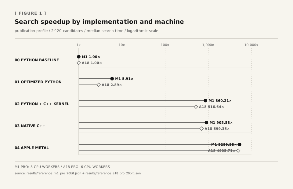
Both machines show the same broad ladder, but not identical gains. Optimized Python reaches 5.91x on the M1 Pro and 2.89x on the A18 Pro. The Python/C++ kernel reaches 860.21x and 516.64x respectively. Metal is much closer across the two machines at 5,289.58x and 4,905.71x. Core topology, scheduling and setup behavior are part of the result, not noise to edit out.
Here are the exact M1 Pro summaries. Values in parentheses are MAD, not standard deviation.
| Stage | Search median (MAD) | vs. baseline |
|---|---|---|
| Python baseline | 16.6223s (0.1150s) | 1.00x |
| Optimized Python | 2.8118s (0.0471s) | 5.91x |
| Python + C++ kernel | 0.0193s (0.0018s) | 860.21x |
| Native C++ | 0.0184s (0.0010s) | 905.58x |
| Apple Metal | 0.0031s (0.0002s) | 5,289.58x |
| Stage | Wall median (MAD) | vs. baseline |
|---|---|---|
| Python baseline | 16.6690s (0.1185s) | 1.00x |
| Optimized Python | 2.9717s (0.0423s) | 5.61x |
| Python + C++ kernel | 0.0644s (0.0011s) | 258.80x |
| Native C++ | 0.0228s (0.0015s) | 730.92x |
| Apple Metal | 0.0445s (0.0010s) | 374.42x |
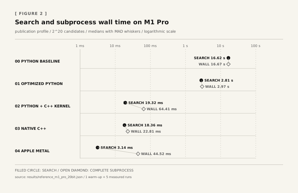
The second plot is the reason I keep both clocks. Metal performs the search in 3.14 milliseconds, but the complete subprocess takes 44.52 milliseconds. Native C++ searches more slowly at 18.36 milliseconds yet finishes the process in 22.81 milliseconds. For this one-shot, one-million-candidate invocation, pipeline and process setup cost more than Metal saves.
That is not a Metal failure. It is a workload-size result. A larger search, a batch of blocks, a persistent process that reuses the pipeline, or a different kernel could amortize setup and reverse the wall-time ranking. Conversely, a tiny search could make parallel Python slower than the scalar baseline. Speedup is always a ratio against a specific baseline on specific hardware under a specific measurement contract.
Reproduce the experiment
The repository targets Apple-silicon macOS and requires Python 3.11 or newer, Clang and the Metal command-line tools. Its README documents the prerequisites and the sanitized results.
make doctor
make all
make test
python3 benchmark.py --profile publication
Each stage’s DESCRIPTION.md contains a reproduction prompt for generating the next implementation while preserving the contract: baseline Python, optimized Python, native kernel, native program and Metal. The checked-in M1 Pro and A18 Pro reports make it possible to inspect the evidence without owning either machine.
Where I stop climbing
There is no universally correct stopping point. My decision is based on the actual way the code is used:
| Stage | Reach for it when | New cost to accept |
|---|---|---|
| Better Python | The algorithm and interpreter hot loop still have obvious waste | More specialized, less general code |
| Parallel Python | Work partitions cleanly and lasts long enough to repay process overhead | Startup, IPC and multi-process debugging |
| Native kernel | A stable, coarse hot path dominates an otherwise useful Python program | ABI, compiler and memory-safety boundary |
| Native program | Python orchestration or deployment is now a measured cost | Larger rewrite and less Python flexibility |
| Metal | There is enough independent work to amortize GPU setup and transfer | New host/shader toolchain and GPU debugging |
I also ask the agent to look for an algorithmic or data-layout improvement before translating the same poor algorithm into a faster language. Existing vectorized libraries may already contain a mature native implementation. I do not want a bespoke shader when one call to a well-tested library solves the real problem.
The famous “premature optimization” line is often used to end this discussion too early. The surrounding argument in Knuth’s Structured Programming with go to Statements is more useful: most small efficiencies are not worth the trouble, but critical code should be identified with measurement and examined carefully. The agentic ladder follows that advice. It leaves ordinary Python alone and makes the critical few percent easier to improve once it has been found.
“Fast enough” is a successful outcome at every stage. If optimized Python reduces a nightly backtest from an hour to ten minutes and the result is ready before I need it, I may prefer that over owning a native extension. If an interactive reverse-engineering tool still freezes for three seconds, a C++ kernel may be justified. If a local key-auditing job would take days, the GPU experiment becomes attractive.
Applying the pattern elsewhere
The XTEA search is intentionally narrow, but the shape appears in many of my workloads:
- A reverse-engineering script may decompress thousands of buffers, emulate a transformation for many candidate configurations or scan independent offsets.
- A cryptographic analysis may evaluate independent keys, nonces or differential candidates against a known oracle.
- A financial backtest may evaluate many parameter sets, instruments or independent windows using the same stable kernel.
- A simulation may run the same state transition for a large batch of independent starting conditions.
The best candidates have four properties: a trustworthy reference implementation, a measurable hot path, work that can be partitioned, and enough repeated computation to pay for the next boundary. The pattern is less useful for I/O-bound programs, tiny one-off operations, tightly sequential algorithms or workloads dominated by moving data rather than computing on it.
Agents make exploring the boundary delightfully easy. I can ask for a multiprocessing version, see that process startup consumes the gain, and discard it. I can ask for a coarse C ABI without committing the rest of the application to C++. I can compare a native binary with the hybrid and learn that their kernels are already at the same plateau. I can ask for a Metal port and discover that the GPU wins only after setup is amortized. A negative result still tells me where to stop.
This is why I think of the approach as a design pattern rather than a one-off optimization trick. Start with code I trust. Wait for a real need. Give the agent a narrow performance contract. Advance by one stage. Keep the result only when it remains correct and improves the metric that matters. Modern coding agents make the ladder easy to try; they do not require every program to reach the top.