In 2020, one of my triage tools printed a file’s entropy as forty colored dots. I mainly used it on executables that might be packed. It was fast, pleasantly colorful and easy to overread.
The dots never proved packing. What helped was seeing where the byte distribution changed. Six years later, I wanted the same quick view with real offsets and without the fake verdict.
The original forty dots
The core of the old tool was small. It divided the file into forty chunks and colored each chunk by its Shannon entropy:
def entropy(s):
    l = float(len(s))
    return -sum(map(lambda a: (a/l)*math.log2(a/l), Counter(s).values()))


def visualize_compression(file_path, bin_count=40):
    with open(file_path, "rb") as f:
        data = f.read()
        chunk_size = int(len(data) / float(bin_count))
        bins = []
        current_chunk = 0
        while current_chunk < len(data):
            ent = entropy(data[current_chunk:current_chunk + chunk_size])
            if ent < 5:
                bins.append(colored('.', 'green'))
            elif ent < 7:
                bins.append(colored('.', 'yellow'))
            else:
                bins.append(colored('.', 'red'))
            current_chunk += chunk_size
        return bins
It did the job in the usual quick-and-dirty RE fashion: read the complete file, chop it into chunks and print some dots. It also gets stuck on files shorter than forty bytes because chunk_size becomes zero. The bigger problem is the color scheme. Two arbitrary thresholds look surprisingly authoritative when they are green, yellow and red.
Forty bins were another shortcut. A tiny executable and a multi-gigabyte image got the same number of dots, even though each dot represented a wildly different amount of data.
A companion packed() helper went further and returned Packed, Possibly packed or Not packed. Its score included sections without raw data and sections with entropy below 1 or above 7. Those are all reasons to look closer at a PE file. They are not specific to packers. Compilers, linkers, installers and ordinary resources can produce the same measurements.
The measurement itself is still useful. Claude Shannon defined entropy from the probabilities of symbols. For bytes, it is calculated as H(X) = -sum(p(x) * log2(p(x))). One repeated byte gives 0 bits per byte. An even distribution of all 256 byte values gives 8.
Bin size really matters. A 128-byte bin cannot contain all 256 byte values, so it cannot reach 8 bits per byte. Larger bins give steadier numbers but hide small transitions. The output needs to show that resolution.
I kept the new display to one strip:
0x00000000 │▁▁▂▂▃▄▅▆▇█│ 0x00090000
            low entropy                    high entropy
A sparkline with byte offsets
The new entropy-map is still one Python file and uses only the standard library. It scans the selected range once through a bounded buffer. Every byte belongs to exactly one bin, and the output prints both the bin size and the half-open file range.
For a predictable demo, I asked OpenAI’s Codex to generate a file with nine 64 KiB regions. The first region repeats one byte, the second alternates two values, and the last cycles through all 256 values. Their entropies run from exactly 0 to 8 bits per byte.
Using eight bins per region makes the staircase obvious in both the block height and the color:
$ python3 entropy/entropy_map.py --bins 72 entropy-demo.bin
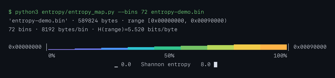
The same output without ANSI color remains readable:
'entropy-demo.bin' · 589824 bytes · range [0x00000000, 0x00090000)
72 bins · 8192 bytes/bin · H(range)=5.520 bits/byte

0x00000000 │▁▁▁▁▁▁▁▁▂▂▂▂▂▂▂▂▃▃▃▃▃▃▃▃▄▄▄▄▄▄▄▄▅▅▅▅▅▅▅▅▆▆▆▆▆▆▆▆▇▇▇▇▇▇▇▇████████████████│ 0x00090000
            0%                                 50%                              100%
                                ▁ 0.0   Shannon entropy   8.0 █
H(range) is 5.520, not the average of the nine local values. It describes the combined byte distribution. The strip shows what happens inside that range. To zoom in, --offset 0x20000 --length 0x30000 --bins 24 selects exactly [0x20000, 0x50000).
Where it fits
There are already existing entropy visualizers. Entroplot uses fixed 1,024-byte blocks and writes a PNG line chart. Binwalk combines an offset-based graph with firmware signatures and extraction. ImHex has an interactive graph and a local-entropy minimap in its hex editor. The archived Veles offers a much broader set of interactive statistical views.
I wanted something simpler: run it in the shell (including using it in ranger or a similar terminal file manager), get a quick map and continue working. There is no GUI, plotting dependency or output file. Give it a file or a byte range and it prints the offsets, resolution and entropy strip.
I read the strip as a map, not a diagnosis. Low entropy may be padding, text or another repetitive structure. High entropy may be compression, encryption, random data or media that was already compressed. A sharp edge may mark an embedded object or an entirely normal format boundary. Entropy gives me a byte range to inspect next. It still cannot prove packing. Good. That was the point of replacing the old dots.